Freezing rows and columns is an important feature for managing your data, especially if you want to make sure that a certain part of your sheet is always visible. In this article, we will walk you through the process of using Collabora’s freeze feature to enhance your data management skills.
Understanding the Basics: Freezing the First Row of a Table
Freezing rows and columns is a popular formatting option. This feature is perfect if you want to be sure that the first row is always visible. To use the Freeze feature for this purpose:
- Go to the View tab.
- Choose Freeze First Row – as you scroll down the column, the first row will remain visible.
- To unfreeze it again, click Freeze Rows and Columns, and it will remove the frozen row.

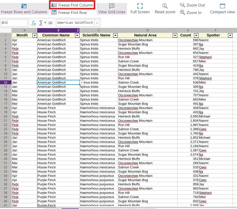
Freezing the First Column of a Table
To freeze the first column, it is ultimately the same as freezing the first row.
- Go to the View tab.
- Choose Freeze First Column – as you scroll down the column, the first column will remain visible.
- To unfreeze it again, click Freeze Rows and Columns, and it will remove the frozen column.
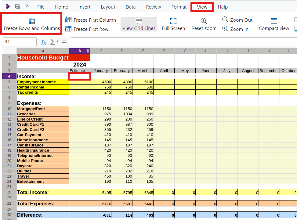
Freezing Rows and Columns Simultaneously
If, for example, you want the top three rows and the first column to always be visible, it’s something you can easily do:
- Put the cursor in the cell just below the rows and to the right of the column you want to freeze.
- Then, simply click Freeze Rows and Columns.
- You’ll notice that as you scroll far to the right, the first column remains visible; also, as you scroll down, the first three rows remain visible.
Keep an eye out for future tips on how to work faster and smarter with your data!